Superposition and field maps

Build a small array by translating one cuboid. The arrangement field is the sum of its members. Sample a plane below the magnets, safely outside all material.

import numpy as np

from microcubed import Arrangement, Magnet

cube = Magnet([80, 80, 40], [0, 0, 0], [0, 0, 8e5])
magnets = [cube.moved_to([x, 0, 0]) for x in (-150, 0, 150)]
array = Arrangement(magnets)
points = np.array([[0, 0, -100], [100, 25, -100]]).T
field = array.Bfield(points)

Verify the result

These assertions also run in GitHub Actions.

np.testing.assert_allclose(field, sum(m.Bfield(points) for m in magnets), atol=1e-14)
np.testing.assert_allclose(array.dBfield(points), sum(m.dBfield(points) for m in magnets), atol=1e-14)
assert np.isfinite(field).all()

Visualize the field and source geometry

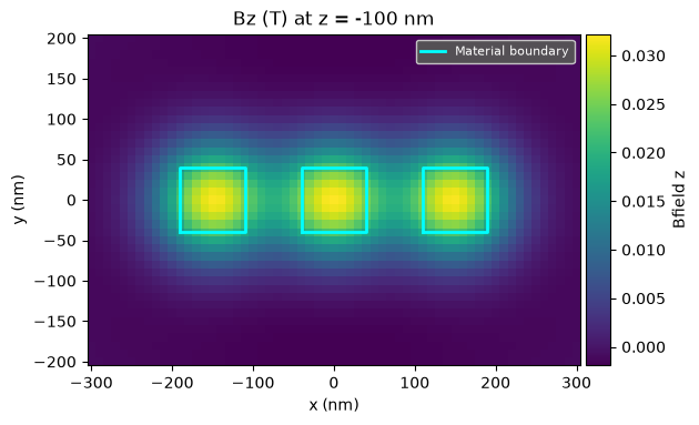
The outlines are XY projections of the source cuboids onto the field map, not intersections with the sampling plane. The cyan line is the projected material boundary, preserving visible gaps and concave boundaries.

import matplotlib.pyplot as plt

fig, ax = array.plot_2d(x=(-300, 300, 61), y=(-200, 200, 41), z=-100, component="z")
for index, boundary in enumerate(array.union_boundary("xy")):
    ax.plot(*boundary, color="#00ffff", linewidth=2, label="Material boundary" if index == 0 else None)
ax.set(xlabel="x (nm)", ylabel="y (nm)", title="Bz (T) at z = -100 nm", aspect="equal")
ax.legend(loc="upper right", fontsize=8, facecolor="#555555", labelcolor="white", framealpha=0.95)
fig.tight_layout()
plt.show()

Line profiles

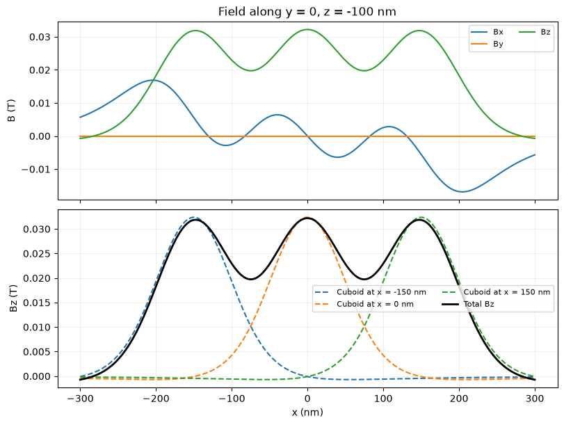
Sample the same exterior line at y = 0, z = -100 nm. The upper panel shows all three field components. The lower panel separates the individual cuboids’ Bz contributions and their sum, making superposition visible.

line_x = np.linspace(-300, 300, 201)
line_points = np.vstack([line_x, np.zeros_like(line_x), np.full_like(line_x, -100)])
line_field = array.Bfield(line_points)
fig, axes = plt.subplots(2, 1, figsize=(8, 6), sharex=True, layout="constrained")
for component, label in enumerate("xyz"):
    axes[0].plot(line_x, line_field[component], label=f"B{label}")
axes[0].set(ylabel="B (T)", title="Field along y = 0, z = -100 nm")
contributions = np.stack([magnet.Bfield(line_points) for magnet in magnets])
for magnet, contribution in zip(magnets, contributions):
    axes[1].plot(line_x, contribution[2], "--", label=f"Cuboid at x = {magnet.center.ravel()[0]:g} nm")
axes[1].plot(line_x, line_field[2], color="black", linewidth=2, label="Total Bz")
axes[1].set(xlabel="x (nm)", ylabel="Bz (T)")
np.testing.assert_allclose(contributions.sum(axis=0), line_field, atol=1e-14)
assert np.isfinite(line_field).all()
for ax in axes:
    ax.grid(alpha=0.2)
    ax.legend(fontsize=8, ncol=2)
plt.show()

3D field and source geometry

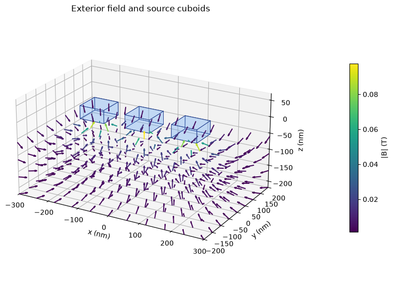
The arrows sample only the exterior region below the cuboids. Arrow direction shows the field direction; color represents its magnitude in tesla. Arrow lengths are normalized for readability, so they do not encode strength. Translucent blue surfaces show the actual cuboid faces at their actual positions.

from mpl_toolkits.mplot3d.art3d import Poly3DCollection

fig = plt.figure(figsize=(9, 6))
ax = fig.add_subplot(projection="3d")
array.plot_3d(
    x=(-300, 300, 11),
    y=(-200, 200, 9),
    z=(-220, -60, 4),
    max_points=396,
    normalize=True,
    length=25,
    ax=ax,
)
for magnet in magnets:
    faces = magnet.corners.T[[[0, 1, 3, 2], [4, 5, 7, 6], [0, 1, 5, 4], [2, 3, 7, 6], [0, 2, 6, 4], [1, 3, 7, 5]]]
    ax.add_collection3d(
        Poly3DCollection(
            faces,
            facecolor="#60a5fa",
            edgecolor="#1e3a8a",
            linewidth=0.6,
            alpha=0.18,
        )
    )
ax.set(
    xlim=(-300, 300),
    ylim=(-200, 200),
    zlim=(-220, 70),
    xlabel="x (nm)",
    ylabel="y (nm)",
    zlabel="z (nm)",
    title="Exterior field and source cuboids",
)
ax.set_box_aspect((600, 400, 290))
ax.view_init(elev=22, azim=-60)
ax.set_position([0.01, 0.06, 0.7, 0.88])
fig.axes[-1].set_position([0.88, 0.22, 0.025, 0.56])
fig.axes[-1].set_ylabel("|B| (T)")
plt.show()