Resolving a polygon boundary

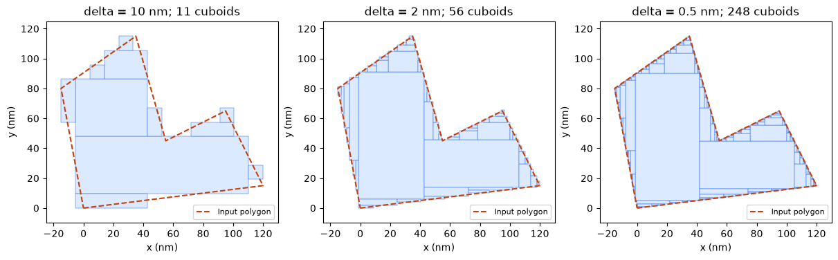
A concave polygon with slanted edges makes rasterization error visible. All lengths are in nm. delta limits the raster-cell size, not the size of the final cuboids: merging adjacent occupied cells into larger cuboids preserves the rasterized geometry exactly. Refining delta improves the staircase approximation along oblique edges. The previous axis-aligned L-shape could be represented exactly by two large cuboids; a small cuboid count alone does not imply a coarse approximation.

import numpy as np

from microcubed import cuboidize

polygon = np.array([(0, 0), (120, 15), (95, 65), (55, 45), (35, 115), (-15, 80)])
thickness = 20
magnetization = [0, 0, 8e5]
delta = 0.5
shape = cuboidize(polygon, t=thickness, delta=delta, mag=magnetization)
field = shape.Bfield([50, 50, -60])
print(f"Raster spacing: {delta} nm; merged cuboids: {len(shape)}")
print("Field at (50, 50, -60) nm (T):", field.ravel())

Raster spacing: 0.5 nm; merged cuboids: 248
Field at (50, 50, -60) nm (T): [-0.00920275 -0.00701831  0.04365604]

Compare boundary resolution

The orange dashed curve is the input polygon. Blue rectangles are projected cuboids, including their internal boundaries. Compare the staircase error at 10 nm, 2 nm, and 0.5 nm; large rectangles in the interior are an exact compression of occupied cells, not a loss of resolution.

import matplotlib.pyplot as plt
from matplotlib.patches import Polygon

closed_polygon = np.vstack([polygon, polygon[0]])
fig, axes = plt.subplots(1, 3, figsize=(12, 4.5), layout="constrained")
for ax, spacing in zip(axes, (10, 2, delta)):
    model = shape if spacing == delta else cuboidize(polygon, t=thickness, delta=spacing, mag=magnetization)
    for cuboid in model:
        ax.add_patch(
            Polygon(cuboid.union_boundary("xy")[0].T, facecolor="#dbeafe", edgecolor="#2563eb", linewidth=0.35)
        )
    ax.plot(*closed_polygon.T, color="#c2410c", linestyle="--", linewidth=1.5, label="Input polygon")
    ax.set(
        xlim=(-25, 130),
        ylim=(-10, 125),
        aspect="equal",
        xlabel="x (nm)",
        ylabel="y (nm)",
        title=f"delta = {spacing:g} nm; {len(model)} cuboids",
    )
    ax.legend(fontsize=8, loc="lower right")
plt.show()

Check field convergence

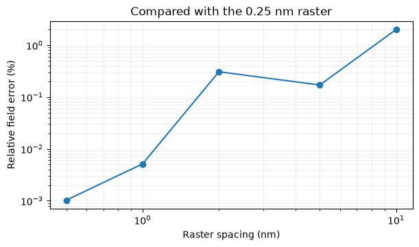
Evaluate identical exterior points for every resolution. The reference uses delta = 0.25 nm; it is a finer raster approximation, not an exact polygon solution. The relative error below is the RMS vector-field difference divided by the reference RMS vector-field magnitude. Raster errors need not decrease monotonically at every step. Area error and field error measure different properties; repeat this check at the observation distances needed for your application.

probe_x = np.linspace(-25, 130, 81)
probes = np.vstack([probe_x, np.full_like(probe_x, 45), np.full_like(probe_x, -60)])
reference = cuboidize(polygon, t=thickness, delta=0.25, mag=magnetization).Bfield(probes)
reference_norm = np.linalg.norm(reference)
polygon_area = (
    abs(np.dot(polygon[:, 0], np.roll(polygon[:, 1], -1)) - np.dot(polygon[:, 1], np.roll(polygon[:, 0], -1))) / 2
)
errors = []
print("delta (nm) | cuboids | area error (%) | relative field error (%)")
for spacing in (10, 5, 2, 1, delta):
    model = shape if spacing == delta else cuboidize(polygon, t=thickness, delta=spacing, mag=magnetization)
    values = model.Bfield(probes)
    area = sum(np.prod(m.size.ravel()[:2]) for m in model)
    error = np.linalg.norm(values - reference) / reference_norm
    errors.append(error)
    print(
        f"{spacing:10g} | {len(model):7d} | {100 * abs(area - polygon_area) / polygon_area:14.5f} | {100 * error:24.5f}"
    )
assert np.isfinite(field).all() and np.isfinite(reference).all()
assert np.isfinite(shape.dBfield(probes)).all()
assert errors[-1] < errors[0], "The refined geometry should improve this exterior-field comparison."
fig, ax = plt.subplots(figsize=(6, 3.5), layout="constrained")
ax.loglog((10, 5, 2, 1, delta), np.array(errors) * 100, "o-")
ax.set(xlabel="Raster spacing (nm)", ylabel="Relative field error (%)", title="Compared with the 0.25 nm raster")
ax.grid(which="both", alpha=0.2)
plt.show()

delta (nm) | cuboids | area error (%) | relative field error (%)
        10 |      11 |        2.86697 |                  1.99932
         5 |      23 |        0.00000 |                  0.17036
         2 |      56 |        0.29891 |                  0.30652
         1 |     121 |        0.00000 |                  0.00513

       0.5 |     248 |        0.00000 |                  0.00102

Refined field map and material boundary

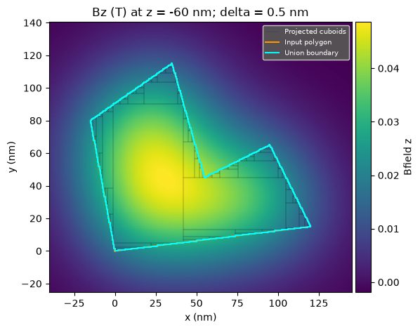
The field is sampled on a 201 × 201 grid at z = -60 nm, below the 20 nm-thick structure. This sampling resolution is independent of the source raster spacing. Thin black lines show the cuboid decomposition; the orange outline marks the input polygon. The cyan union_boundary("xy") follows the actual rasterized material, retaining the notch. It removes internal cuboid edges and returns separate closed loops for disconnected pieces and holes. All outlines are XY projections onto the map.

import matplotlib.pyplot as plt

fig, ax = shape.plot_2d(x=(-40, 145, 201), y=(-25, 140, 201), z=-60, component="z")
for index, cuboid in enumerate(shape):
    ax.plot(
        *cuboid.union_boundary("xy")[0],
        color="black",
        linewidth=0.3,
        alpha=0.35,
        label="Projected cuboids" if index == 0 else None,
    )
ax.plot(*np.vstack([polygon, polygon[0]]).T, color="#ff9500", linewidth=1.5, label="Input polygon")
for index, boundary in enumerate(shape.union_boundary("xy")):
    ax.plot(*boundary, color="#00ffff", linewidth=1.5, label="Union boundary" if index == 0 else None)
ax.set(xlabel="x (nm)", ylabel="y (nm)", title="Bz (T) at z = -60 nm; delta = 0.5 nm", aspect="equal")
ax.legend(loc="upper right", fontsize=7, facecolor="#555555", labelcolor="white", framealpha=0.95)
fig.tight_layout()
plt.show()