Single cuboid

Calculate the field and its analytical gradient outside a uniformly magnetized cube. All lengths here are in nm, magnetization is in A/m, fields are in T, and gradients are in T/nm.

import numpy as np

from microcubed import Magnet

cube = Magnet(size=[100, 100, 100], center=[0, 0, 0], magnetization=[0, 0, 8e5])
points = np.array([[0, 0, -150], [80, 0, -150]]).T
field = cube.Bfield(points)  # (3, N): Bx, By, Bz
gradient = cube.dBfield(points)  # (3, 3, N): derivative axis, field axis, point
print(field)

[[ 0.         -0.02004397]
 [ 0.          0.        ]
 [ 0.04560013  0.02190495]]

Verify the result

These assertions also run in GitHub Actions.

assert field.shape == (3, 2)
assert gradient.shape == (3, 3, 2)
assert np.isfinite(field).all() and np.isfinite(gradient).all()
# Reflection symmetry makes transverse components vanish on the z axis.
np.testing.assert_allclose(field[:2, 0], 0, atol=1e-14)

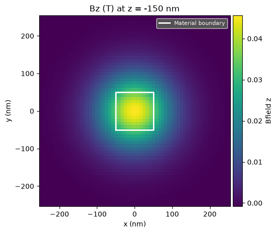
Visualize the field and source geometry

The outlines are XY projections of the source cuboids onto the field map, not intersections with the sampling plane. The white line is the projected material boundary. The cube is above the sampling plane.

import matplotlib.pyplot as plt

fig, ax = cube.plot_2d(x=(-250, 250, 61), y=(-250, 250, 61), z=-150, component="z")
for boundary in cube.union_boundary("xy"):
    ax.plot(*boundary, "w-", linewidth=2, label="Material boundary")
ax.set(xlabel="x (nm)", ylabel="y (nm)", title="Bz (T) at z = -150 nm", aspect="equal")
ax.legend(loc="upper right", fontsize=8, facecolor="#555555", labelcolor="white", framealpha=0.95)
fig.tight_layout()
plt.show()

Line profiles

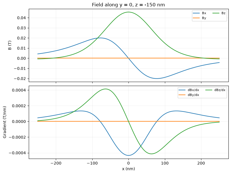
Sample the same exterior line at y = 0, z = -150 nm. The upper panel shows all three field components. The lower panel shows analytical derivatives along the line; these use dBfield(), not finite differences.

line_x = np.linspace(-250, 250, 201)
line_points = np.vstack([line_x, np.zeros_like(line_x), np.full_like(line_x, -150)])
line_field = cube.Bfield(line_points)
fig, axes = plt.subplots(2, 1, figsize=(8, 6), sharex=True, layout="constrained")
for component, label in enumerate("xyz"):
    axes[0].plot(line_x, line_field[component], label=f"B{label}")
axes[0].set(ylabel="B (T)", title="Field along y = 0, z = -150 nm")
line_gradient = cube.dBfield(line_points)
for component, label in enumerate("xyz"):
    axes[1].plot(line_x, line_gradient[0, component], label=f"dB{label}/dx")
axes[1].set(xlabel="x (nm)", ylabel="Gradient (T/nm)")
assert np.isfinite(line_gradient).all()
assert np.isfinite(line_field).all()
for ax in axes:
    ax.grid(alpha=0.2)
    ax.legend(fontsize=8, ncol=2)
plt.show()

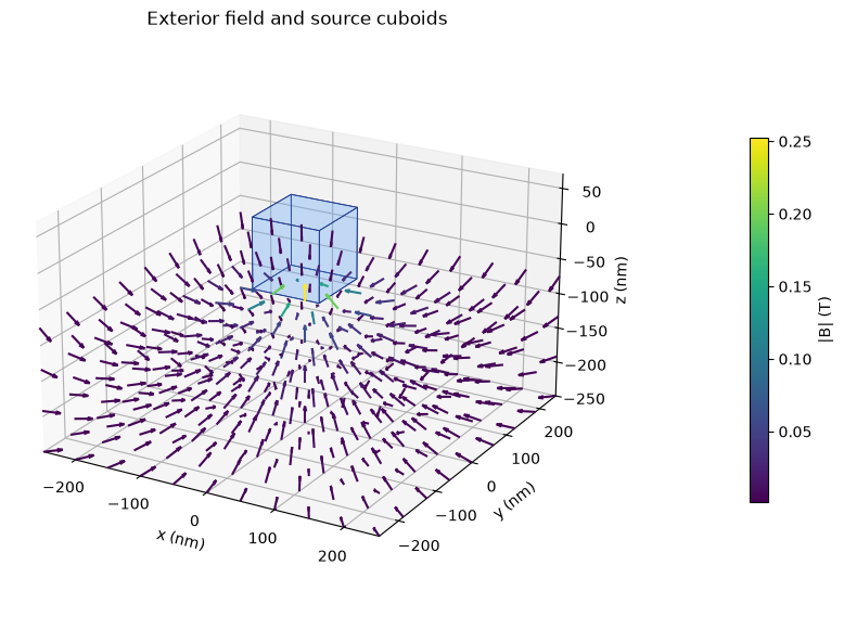
3D field and source geometry

The arrows sample only the exterior region below the cuboids. Arrow direction shows the field direction; color represents its magnitude in tesla. Arrow lengths are normalized for readability, so they do not encode strength. Translucent blue surfaces show the cuboid faces at their actual position.

from mpl_toolkits.mplot3d.art3d import Poly3DCollection

fig = plt.figure(figsize=(9, 6))
ax = fig.add_subplot(projection="3d")
cube.plot_3d(
    x=(-250, 250, 11),
    y=(-250, 250, 9),
    z=(-250, -75, 4),
    max_points=396,
    normalize=True,
    length=25,
    ax=ax,
)
for magnet in [cube]:
    faces = magnet.corners.T[[[0, 1, 3, 2], [4, 5, 7, 6], [0, 1, 5, 4], [2, 3, 7, 6], [0, 2, 6, 4], [1, 3, 7, 5]]]
    ax.add_collection3d(
        Poly3DCollection(
            faces,
            facecolor="#60a5fa",
            edgecolor="#1e3a8a",
            linewidth=0.6,
            alpha=0.18,
        )
    )
ax.set(
    xlim=(-250, 250),
    ylim=(-250, 250),
    zlim=(-250, 70),
    xlabel="x (nm)",
    ylabel="y (nm)",
    zlabel="z (nm)",
    title="Exterior field and source cuboids",
)
ax.set_box_aspect((500, 500, 320))
ax.view_init(elev=22, azim=-60)
ax.set_position([0.01, 0.06, 0.7, 0.88])
fig.axes[-1].set_position([0.88, 0.22, 0.025, 0.56])
fig.axes[-1].set_ylabel("|B| (T)")
plt.show()