Calculating fields and gradients

Magnetic flux density \(\mathbf B\)

import numpy as np
from microcubed import Magnet

bar = Magnet([500, 300, 50], [0, 0, 0], [1.467e6, 0, 0])
x = np.linspace(-500, 500, 201)
points = np.vstack([x, np.zeros_like(x), -150 * np.ones_like(x)])

B = bar.Bfield(points)
Bx, By, Bz = B
print("Field shape:", B.shape)
print("Field at the middle of the line (T):", B[:, len(x) // 2])

Field shape: (3, 201)
Field at the middle of the line (T): [-0.03951034  0.          0.        ]

B.shape == (3, N). The coordinate order is always (x, y, z).

Magnetic field strength \(\mathbf H\)

H = bar.Hfield(points)
print("H at the middle of the line (A/m):", H[:, len(x) // 2])

H at the middle of the line (A/m): [-31441.32676077      0.              0.        ]

In the exterior-medium model, \(\mathbf H=\mathbf B/\mu_0\).

Analytical gradient

dB = bar.dBfield(points)

dxBx = dB[0, 0]
dxBy = dB[0, 1]
dxBz = dB[0, 2]
dyBx = dB[1, 0]
dzBz = dB[2, 2]
print("Gradient shape:", dB.shape)
print("Maximum |dBx/dx| (T/nm):", np.max(np.abs(dxBx)))

Gradient shape: (3, 3, 201)
Maximum |dBx/dx| (T/nm): 0.0005041552418873724

dB.shape == (3, 3, N). For geometry in nm, its unit is T/nm.

Quantities parallel and perpendicular to an \(x\)-directed magnetisation can, for example, be defined as

G_parallel = np.abs(dB[0, 0])
G_perpendicular = np.hypot(dB[0, 1], dB[0, 2])

Analytical or finite-difference gradients?

Use dBfield() for gradients in Microcubed calculations. Finite differences of Bfield() are useful as a diagnostic when comparing against a grid-based solver: applying the same stencil to both fields separates field disagreement from numerical derivative approximation error. They are not a separate field solver and require a choice of step size.

The Ubermag/OOMMF comparison explains this error decomposition and reports both comparisons. Its optional execution produces current error ranges rather than fixed benchmark claims.

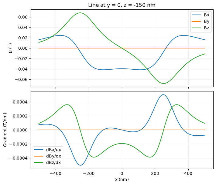
Field and gradient along the line

import matplotlib.pyplot as plt

fig, axes = plt.subplots(2, 1, figsize=(7, 6), sharex=True, constrained_layout=True)
for i, name in enumerate("xyz"):
    axes[0].plot(x, B[i], label=f"B{name}")
    axes[1].plot(x, dB[0, i], label=f"dB{name}/dx")
axes[0].set(ylabel="B (T)", title="Line at y = 0, z = -150 nm")
axes[1].set(xlabel="x (nm)", ylabel="Gradient (T/nm)")
for ax in axes:
    ax.legend()
    ax.grid(alpha=0.2)
plt.show()

Sampling a region without plotting

sample_field accepts either a fixed value or (start, stop, count) for each axis:

from microcubed import sample_field

(x, y, z), field = sample_field(
    bar,
    x=(-450, 450, 101),
    y=(-350, 350, 81),
    z=-150,
    what="Bfield",
)

print(field.shape)  # (3, 101, 81, 1)

(3, 101, 81, 1)

All three spatial axes are retained, including axes of length one. For gradients:

coordinates, gradient = sample_field(
    bar,
    x=(-450, 450, 101),
    y=(-350, 350, 81),
    z=-150,
    what="dBfield",
)

print(gradient.shape)  # (3, 3, 101, 81, 1)

(3, 3, 101, 81, 1)

Direct call syntax

Magnets and arrangements are also callable:

B_grid = bar((-450, 450, 101), (-350, 350, 81), -150, what="B")
dB_grid = bar((-450, 450, 101), (-350, 350, 81), -150, what="dB")

For new code, sample_field is recommended because coordinates and results are returned together without squeeze.

Interior points and surfaces

Magnet.Bfield and Magnet.dBfield return NaN for interior and boundary points. This prevents the exterior formulation from being interpreted as a material model inadvertently.

For Arrangement, checking every point against every cuboid is intentionally omitted for performance. If a sampling grid intersects magnets, construct an explicit mask from their bbox values.